Simulate, Test, Analyze: A Framework For Rigor

trebuchet-launch---08_23970235271_o

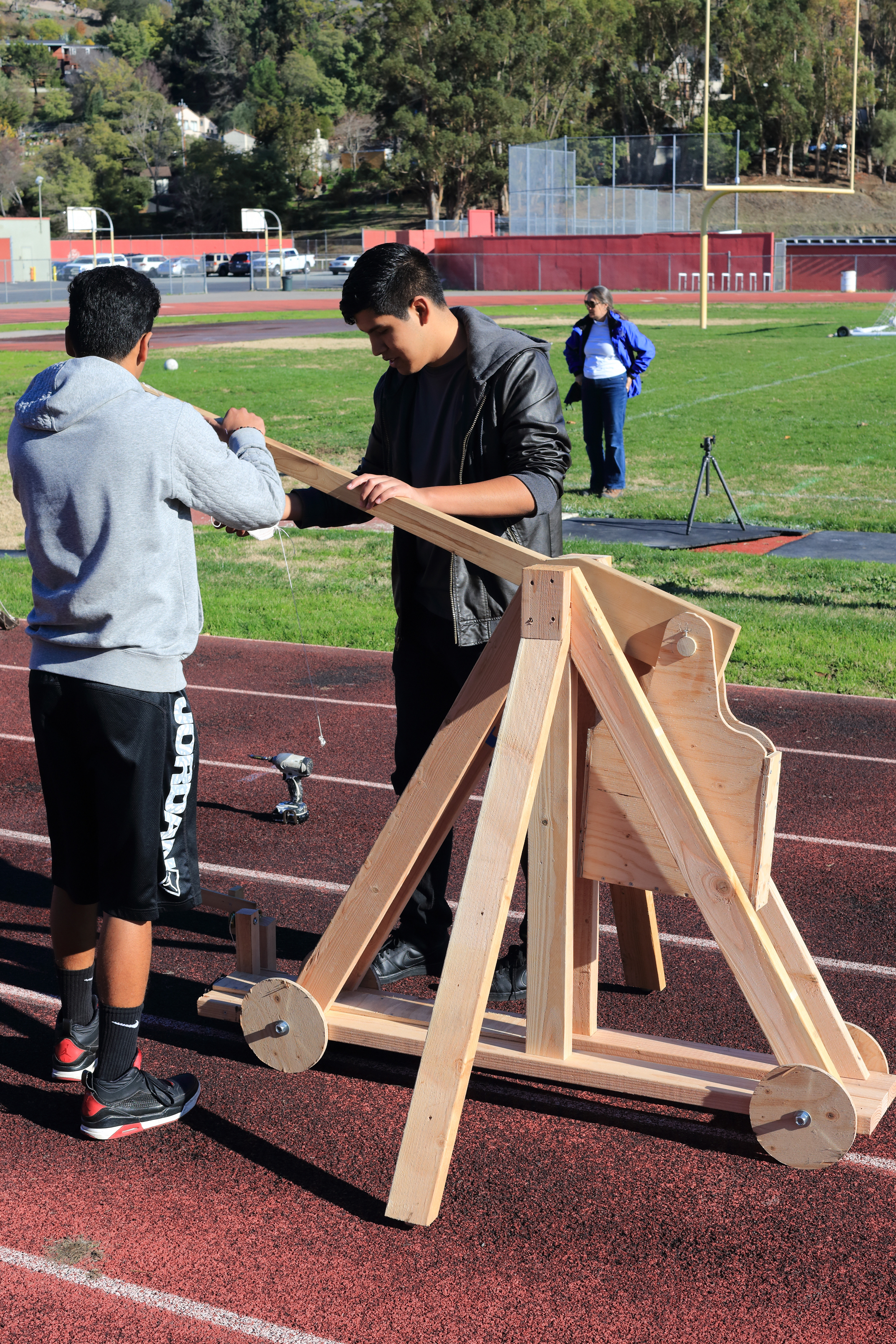
“Have Fun Storming The Castle!”

At the end of this fall semester, the second year students in the Academy rolled and carried their medieval mechanisms of mayhem to the SRHS track and we spent the afternoon watching the devices hurl lacrosse balls across the athletic field.This project was the final performance assessment of the semester and required that students design a gravitationally powered projectile launcher. This is an age old engineering/applied physics project.

Like many engineering projects done in high school, the physics principles governing the dynamics of the project are quite complicated, and ultimately the actual “application” of the science principles is often cursory. Students don’t have the background or mathematical abilities to to do the complex calculations needed to make an optimization adjustment to their mechanical device.This leads to the disconnection between the science content and engineering practice. Students don’t have the ability to make an informed decision about design choices. This is because it is difficult, very difficult.

Over the past few years I have been very interested in addressing this problem. This post discusses a framework that I have been working on to incorporate science into engineering projects. I think this framework allows high school students to engage in difficult scientific analysis without overwhelming them.

A Framework For Rigor

I won’t claim that this is a perfect solution, but so far I think we have experienced some success in creating a tighter relationship between science and engineering.  Last December I helped conduct a workshop at the NCCPA Professional Development Conference in Petaluma, CA. The name of the workshop was “NGSS, Prediction Reports and Your Science Class” and the point of this workshop was to give the attendees a framework for incorporating the Engineering standards into the science curriculum.  My co-presenter (Vipul Gupta) and I focused on the creation of prediction reports using computer simulations as a way to address two very important standards in the NGSS framework:

Using Simulations with Informed Input

Computer simulations are very popular in the educational space. They give teachers and students a virtual space where students can interact with virtual lab equipment or virtual objects that behave similarly to physical objects in the real world. With that said, they can fail to address students misconceptions because they do not always succeed in linking a conceptual model to the physical behavior. I also believe that the best simulations are ones that output data that can be analyzed with other scientific/mathematical tools. I also think that a good simulation requires that students provide meaningful input that gives them opportunities for analyzing the relationship between the input and the output.

Simulations used in engineering projects can be extremely helpful in addressing one of the main problems in engineering education. Students often design and build mechanical devices without understanding the physical principles that govern the design. The design process becomes an exercise in trial and error, or simply is reduced to copying a design from the internet.

To do a predictive analysis of a rocket’s flight, or a bridge’s structural performance is extremely difficult and often requires advanced mathematics and physics. Simulations can give the students the ability to analyze their designs and understand how changing the design inputs affects the output. Once again, it is important to find a simulation that requires students to understand the inputs and outputs.

Virtual Trebuchet

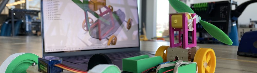
For example, in our project, students were introduced to an online Trebuchet simulation tool. This simulation tool is great because it requires that the student learn how to measure and calculate certain inputs. The students must have a working knowledge of rotational inertia, center of mass, and other concepts before they use the simulation. This was ideal for our project because it gave students a relevance and motivation . They had learn about these concepts in order to actually use the simulation. The students could then change certain inputs and see how that would change the efficiency of the design, or the range of the projectile. The point is that they needed physics knowledge in order to use the tool. They might not have the ability to know how the simulation eventually calculated the output, but they knew that the simulation required an understanding of the inputs.

IMG_2674

Example Report

The Prediction Report

The next step is to ask the students to prepare a prediction report. This report is designed to get students to demonstrate their understanding of the inputs, display evidence of the required calculations or measurements needed to create the inputs and then analyze the simulation outputs. In the report for this project, I asked students to show a set of calculations and measurements for determining the center of mass of their throwing arm and the rotational inertia (moment of inertia). Students also had to provide similar information for the counterweight.  The students then had to run the simulation and document the outputs from the simulation.

The Test:  Data is Needed

The next step is to test the device. To make this step more rigorous and to be able to relate the scientific analytical process to the engineering process, it is crucial for the students to collect data that can be used to analyze the performance of their device/product and then reflect on how they would improve their design.

For this project, we decided to use high-speed video and Vernier’s LoggerPro video analysis software to plot the position of the projectile as it was launched from the device.

The Analysis

The analysis is actually broken into two parts. The first part requires a collection of calculations while the second part uses those calculations to make some qualitative assessments.

For example, in the above project, students had to use the collected position data from the video analysis tool to calculate the kinetic energy of the projectile and then the efficiency of the device. They had to be proficient at the analytical tool, which in itself requires physics content knowledge, providing once again an opportunity to apply scientific models in the analysis portion of this engineering project.

I have included the instructions for the analysis report here: Projectile Launcher Analysis Report.

Finally, students are given the opportunity to use the information gathered in the analysis report to reflect on their design, and more importantly use the information to inform how they would improve on a future design. I have included below the set of questions that I asked my students:

  1. Compare the efficiency calculation of the simulation to the efficiency rating that you calculated for your actual performance. Please describe why you think these values are not the same.
  2. Consider the design of your trigger. What design and fabrication decisions would you change in order to improve your trigger, AND explain WHY you would make those changes.
  3.  Consider the design of your sling. What design and fabrication decisions would you change in order to improve your sling, AND explain WHY you would make those changes.
  4. Consider the design of your release mechanism (called the nose). What design and fabrication decisions would you change in order to improve this mechanism, AND explain WHY you would make those changes.
  5. Consider the design of your arm. What design and fabrication decisions would you change in order to improve your arm, AND explain WHY you would make those changes.
  6. Consider the design of all other components and the overall design. What design and fabrication decisions would you change in order to improve your device (other than the trigger, sling and arm), AND explain WHY you would make those changes.

Conclusion

The overall design of this framework can be boiled down to this:

  • Engage students in a computer simulation that simplifies the process of modeling and analyzing a complex physical/chemical/biological process, but be sure that the simulation requires some conceptual and computational thinking.
  • When testing the performance of the design (bridge, rocket, etc.) make sure that the students are required to  collect data that can be analyzed and that once again demands that they apply their theoretical models.
  • Design an assessment that uses the analysis and gives the students an opportunity to make informed judgements of their designs for the purpose of redesign.

Testing Motors For The Solar Dragster Race

Torque/Speed Curves

In this post I’m going to describe our attempt to measure the power curve for the DC motors used in the Solar Dragster race this year. I’m going to be honest, our efforts weren’t really that successful, but I can at least say that I learned some things that might help for next year, and I think the students were able to do some authentic device testing – a part of being an engineer.

Last year I was a bit concerned that the DC motors that we were using in the Solar Dragster Race were not actually outputting the same power. I wanted to devise a way to measure the motor power, and then have each team do their own analysis. I wanted the students to do this without understanding the electrical power parameters involved because we were at this point only looking at motors as being a black box that gets energy from a source and transfers that energy into a rotational device – i.e. an axle, then to a gear, then to another axle, and finally to a wheel. I looked into getting a torque sensor, but quickly found out that these cost a fortune!

I came across this interesting website from MIT, which was a nice resource for the theory about DC motor performance. The site does a nice job in explaining torque/speed curves, and how the graph of torque vs angular speed is essentially linear for DC motors. That meant that all the students really needed to do was to measure stall torque and the no load speed of their motors and then we would have the torque/speed curve. The website identifies a device that they custom built for testing motors, and it looks interesting, but I didn’t have time to reverse engineer what they had built and unfortunately the images and videos aren’t clear enough to easily understand how the device works – something perhaps for summer tinkering…

One of the issues with the little DC motors that you buy is that the arbor is really small, and it has no index, so its really hard to attach anything. Generally, you have to go with a friction fitting, and I was worried that doing a stall torque test was going to be difficult. Mr. Holt and I designed and printed out a little lever arm to attach to the motors. This little arm could then be attached to a force meter to measure the stall torque and then also used to help measure the rotational velocity using a Photogate. The final “test-bench” looked like this:

Torque-speed test bench

The motors were clamped to a lab stand that was then placed so that the little lever arm would rotate and block the Photogate laser as it spun. This is how the students measured the no load speeds. Then they attached a string to the little hole in the arm, and then attached this to a force meter to get the stall torque. All the motors were tested with essentially the same power source – two AA batteries.

I then had the students share their data using a Google Spreadsheet and I compiled the data – here it is on Plotly:

dc_motor_tests

There is obviously some variability in the motor performance, but its hard to tell if any of the motors give a distinctive advantage over the others because I suspect that the data is not that reliable unfortunately. I do suspect that the angular speed data might be inaccurate due to the fact that we were getting some very differing results from the Photogate. Although we made the sampling rate as rapid as possible, I still am not confident that the Photogate was able to read the blocking of the laser accurately – the motors spin VERY fast (upwards of 5000 RPM’s when not loaded). I’m also not sure if the data then could then be used in any instructive way to help students make design decisions about their dragsters.

Although this may seem like a failure, it did allow the students to identify at least two motors that we knew were malfunctioning, so we were able to swap those out before the competition.

For Next Year

I think at this point I would want to make some changes to this activity. Although it was somewhat helpful in giving the students a direct interaction with data associated with the performance of a DC motor, and how that performance is calculated at the product of the torque and angular velocity, I’m not sure that the activity supplied data that was good enough to then use as an input factor in the competition. For example, I didn’t feel confident about allowing students to use the calculated maximum input power as a scaling factor for their dragster race time.

Perhaps next year, we can find the funds to purchase a high precision, digital torque meter, or find the time and money to build our own “analog” torque/speed meter like the one that MIT designed. All in all, I’d say this activity was partially successful.

Building The Net Torque Model – Part 3

Appending The Conservative Models

After investigating the causal relationship between torque and angular acceleration, I introduced the possibility to the class that perhaps we also needed to revisit the Energy Transfer Model and the Momentum Transfer Model. The students agreed that an object that is rotating must have energy. This was pretty easy to demonstrate.

I set up a situation in the class where two of the variable inertia disks that we created on the 3D printers were placed at the top of an inclined ramp. The internal marbles were placed at two different configurations inside the disks and then the students predicted which disk would reach the end of the ramp first. I was pleased to find out that the class appeared to agree that the disk with the marbles located closer to the radius would be the winner. I really think that our investigation with the variable inertia disks solidified the students’ conceptual understanding of rotational inertia and the importance of mass distribution.

I have not yet found a good experiment where students could discover the rotational kinetic energy relationship, so I decided to take them through a derivation based on linear kinetic energy. I then asked the students to do some whiteboard work. I asked them to demonstrate that the disks would indeed reach the end of the ramp at different times. Although this wasn’t strictly a constructivist approach, it was good practice in doing some fairly difficult algebra without numerical values – something the students traditionally are not very good at.

We then moved onto momentum. Again, I started by reviewing the Momentum Transfer Model for a particle. At this point the pattern had been fairly well established. The relationship between angular and linear quantities seemed to have taken hold because the students were quick to propose a mathematical definition for angular momentum. Our next goal was to figure out whether this was a conserved quantity.

Mr Holt and I had created a set of metal disks that could be attached to the rotary sensors. I decided to create our own, rather than (sorry Vernier) buy them as I thought that the commercial kit was over priced. It wasn’t too hard to create the disks, especially when you have access to a CNC plasma cutter!

image1

The students attached one disk to the rotary motion sensor and then got that disk spinning. They then took a second disk that had small magnets attached to it, and dropped this disk onto the spinning disk. The students compared the angular velocity before and after the disks were combined and then calculated the angular momentum of the system before and after. The data we got was quite good with the class getting in the range of only about a 5% to 6% difference.

Wrapping it Up (or Un-Rolling It Down)

As a final deployment, I decided to try the deployment activity that Frank Nochese did with his students. It seemed like a good (and fun) way to wrap up our model (or as I have already argued – models).

Before doing the deployment activity, I reviewed all the model specifics with the students. My point here was to impress on them that what we had not really built a new model, but rather had extended many of the prior particle models to include rigid extended bodies. This generally only required that we consider the moment arm in all the particle models. I think this really helped a number of students see the connection between models that they felt they understood and all this rotational stuff that seemed a bit confusing.

I then set them up with the deployment activity, but I asked them to specifically solve the problem using both energy and net torque. There was some success, but I realized that the task was a bit much for the class. Once again, it is clear that I need to give them more practice with these problems that require multiple steps and that involve algebraic manipulation of symbols without numbers. Plenty of time to practice that!

Building The Net Torque Model – Part 1

A New Model (or Five New Models!)

So, since I decided to incorporate AP Physics into the Academy as the singular curricular pathway for all students, I needed to see what models might need to be added (and mostly removed) from the past curriculum. The big change was to remove the study of thermodynamics and much of magnetism, and add rotation. I hadn’t officially taught rotation since the Academy was first started nine years ago and since I had started using the modeling approach, so I looked at the curriculum AMTA had stored away in its repository. After reading through the material, I honestly have to say I don’t think the American Modeling Teachers Association’s curricular material on the topic of rotational motion is as good as some of the other material they offer. First of all, I have struggled with the idea of teaching this as a unit on Rotational Motion. It seems to go against the modeling approach of defining a distinct model that is either descriptive (kinematic), causal (force), or “conservational” (energy and momentum). The material seemed too similar to the traditional approach. Also, there seems to be some major holes in the curriculum (where are the notes describing the paradigm labs or the deployment practicums?) It would seem that in order to capture rotational motion as an analytical model you would need quite a few models if you were to follow the pattern developed in linear motion. You would need to define a Constant Angular Velocity Particle Model, a Constant Angular Acceleration Particle Model, a Net Torque Model (Net Balanced Torque and Unbalanced Torque), and then either two more models, or at least an addendum to both the Momentum Transfer Model and the Energy Transfer Model. Additionally, each of the linear models refer to the main constituent as a particle. So technically, if I wanted to remain true to the model naming convention, I’d have to use a name like Constant Angular Velocity Rigid Extended Body Model (CAVREBM). That seemed absurd. After some time, I decided to settle on the Net Torque (Rigid Body) Model or NTM. I felt that this model could cover kinematic descriptions, causal relationships between a net torque and a rigid body and then point to how the previous momentum and energy models needed to be adjusted. Here is how we first started to build this model…

Defining Angular Displacement and Angular Velocity

At the outset of our task to build this model, the students did a simple activity where they graphed the angle of rotation of a wooden disk with the distance the disk rolled across a flat surface. When they graphed the angle through which the wheel turned to the distance the wheel rolled, they found that the radius of the wheel was the slope. This meant that the linear displacement of a rolling object could be related to the angular displacement and likewise, the rate of these displacements were related through the radius.

Turning Effect

Once we had established some understanding around angular displacement, we started this model by investigating the conditions under which a rigid body’s rotational motion changed and when it didn’t change. I want to thank Sam for his post on how to begin investigating a turning effect.The students essentially followed this line of questioning and observing to establish a set of rules for defining when a rigid body’s rotational motion state will change. This lead the students to first make the claim that a change in “turning” was due to an unbalanced force acting on the wheel (especially those forces acting at a right angle to the radius!). The “turning” didn’t seem to change much when the forces acting on the wheel were balanced.

Uh, The Forces Aren’t Balanced, But The Thing Isn’t Turning?

The next class, I set up a simply “see-saw” with a meter stick and two different masses placed at different locations so that the meter stick didn’t rotate. I then asked the students if the forces were balanced. They immediately replied – “no”. So what gives? Students immediately saw that the Force Particle Models were not sufficient in dealing with rigid body motion, and many immediately suggested that the distance from the center of rotation also affected the “turning effect”. This discovery lead to a discussion about particles.

Extended Rigid Bodies vs. Particles

All the models that we had built in the past assumed that an object could be simplified by accepting that all the mass of the object could be identified as being located at a single point, namely the center of mass, because each particle of mass located in an object was experiencing the same linear motion state. The problem with a rotating object is that most points within a rotating object are actually traveling with different linear velocities (and accelerations). We needed a new way to define the basic constituent of this model. I suggested that we stick to as simple a definition as possible – a rigid extended body. This could be identified by a straight line (or lines) passing through a rotation point. The length represented an “un-bendable, un-squishable” collection of particles extending from the center of rotation outward to any edge of the extended body.

The Moment For The Moment Arm

This set us up for the next investigation. I asked the students to create an investigation where they had to prove that there was a connection between the force and the location that force was being applied and the turning effect. Students at first struggled to create an investigation that demonstrated a functional (input=output) relationship. Many students found evidence that supported their hypothesis, but I had to explain that these were not conclusive because it was limited to a single data point. This lead to a rich whiteboard session where students worked through the process of designing an experiment that went beyond describing a single situation. I’d like to return to this at a later point regarding scientific reasoning, but that is going to have to wait. Students eventually graphed the output force required when the input distance from the center of rotation was changed – in order for the system’s rotational motion state to be unchanged. This also quickly lead to the question of direction. It seemed that the force direction in relation to the radius of rotation seemed to affect the rotational state of the meter stick. At this point I introduced the concept of Torque and we discussed the vector cross product. I think for future classes, I’d like to introduce the cross product a bit differently. Using the line of action (as is done sometimes by engineers) seems to be a more useful method – at least visually – in explaining why the angle of the force is also part of what defines the torque value.

Deploying The Model (Part 1):

To test the model (thus far), the students were given a meter stick with a small weight attached to one end. The students then had to predict the point at which the meter stick could be moved off the edge of a table before rotating, and thus fall off. This allows the students to see the importance of identifying the gravitational force on the stick as affecting the turning effect around a point of rotation – which in this case was clearly not the center of mass of the stick. After some challenges, the students were mostly able to predict the point at which their meter sticks could be pushed before falling off the table. Next time, I’d like to reinforce this by also doing an experiment where two force meters support a meter stick with weights placed at different locations along the meter stick and have the students predict the forces read by both force meters. It was now time to look at situations where the torques were unbalanced. On to the second part of the model.